── Attaching core tidyverse packages ──────────────────────── tidyverse 2.0.0 ──
✔ dplyr     1.1.4     ✔ readr     2.1.5
✔ forcats   1.0.0     ✔ stringr   1.5.1
✔ ggplot2   3.5.1     ✔ tibble    3.2.1
✔ lubridate 1.9.3     ✔ tidyr     1.3.1
✔ purrr     1.0.2
── Conflicts ────────────────────────────────────────── tidyverse_conflicts() ──
✖ dplyr::filter() masks stats::filter()
✖ dplyr::lag()    masks stats::lag()
ℹ Use the conflicted package (<http://conflicted.r-lib.org/>) to force all conflicts to become errors
library(mosaic)
Registered S3 method overwritten by 'mosaic':
  method                           from
  fortify.SpatialPolygonsDataFrame ggplot2

The 'mosaic' package masks several functions from core packages in order to add
additional features.  The original behavior of these functions should not be affected by this.

Attaching package: 'mosaic'

The following object is masked from 'package:Matrix':

    mean

The following objects are masked from 'package:dplyr':

    count, do, tally

The following object is masked from 'package:purrr':

    cross

The following object is masked from 'package:ggplot2':

    stat

The following objects are masked from 'package:stats':

    binom.test, cor, cor.test, cov, fivenum, IQR, median, prop.test,
    quantile, sd, t.test, var

The following objects are masked from 'package:base':

    max, mean, min, prod, range, sample, sum
library(skimr)
Attaching package: 'skimr'

The following object is masked from 'package:mosaic':

    n_missing
library(ggformula)
Dataset - Gender at the Work Place
This is a dataset pertaining to gender and compensation at the workplace.
Warning: One or more parsing issues, call `problems()` on your data frame for details,
e.g.:
  dat <- vroom(...)
  problems(dat)
Rows: 32 Columns: 1
── Column specification ────────────────────────────────────────────────────────
Delimiter: ","
chr (1): year;occupation;major_category;minor_category;total_workers;workers...

ℹ Use `spec()` to retrieve the full column specification for this data.
ℹ Specify the column types or set `show_col_types = FALSE` to quiet this message.
job_gender
# A tibble: 32 × 1
year;occupation;major_category;minor_category;total_workers;workers_male;wo…¹
<chr>
1 2016;Dietitians and nutritionists;Healthcare Practitioners and Technical;Hea…
2 2016;Medical records and health information technicians;Healthcare Practitio…
3 2016;Pharmacists;Healthcare Practitioners and Technical;Healthcare Practitio…
4 2016;Licensed practical and licensed vocational nurses;Healthcare Practition…
5 2016;Miscellaneous therapists, including exercise physiologists;Healthcare P…
6 2016;Clinical laboratory technologists and technicians;Healthcare Practition…
7 2016;Registered nurses;Healthcare Practitioners and Technical;Healthcare Pra…
8 2016;Nurse practitioners;Healthcare Practitioners and Technical;Healthcare P…
9 2016;Physician assistants;Healthcare Practitioners and Technical;Healthcare …
10 2016;Health practitioner support technologists and technicians;Healthcare Pr…
# ℹ 22 more rows
# ℹ abbreviated name:
# ¹`year;occupation;major_category;minor_category;total_workers;workers_male;workers_female;percent_female;total_earnings;total_earnings_male;total_earnings_female;wage_percent_of_male`
Rows: 32 Columns: 12
── Column specification ────────────────────────────────────────────────────────
Delimiter: ";"
chr (3): occupation, major_category, minor_category
dbl (7): year, total_workers, workers_male, workers_female, total_earnings, ...
num (2): percent_female, wage_percent_of_male

ℹ Use `spec()` to retrieve the full column specification for this data.
ℹ Specify the column types or set `show_col_types = FALSE` to quiet this message.
The dataset includes columns such as total workers, the distribution of male and female workers, total earnings (segregated by gender), and wage comparisons between male and female workers. It categorizes these occupations under a major category called “Healthcare Practitioners and Technical,” which is further divided into specific occupations like dietitians, registered nurses, and nurse practitioners. The dataset highlights gender disparities in these healthcare roles by comparing the number of male and female workers, their respective earnings, and the proportion of female workers in each role. It provides insights into wage differences, showing a column indicating how female earnings compare to male earnings (wage_percent_of_male).
First 10 rows of the Gender at the Work Place dataset
The first ten rows of the “Gender at the Workplace” dataset focus on healthcare-related occupations in 2016. These occupations include roles like “Dietitians and Nutritionists,” “Pharmacists,” and “Registered Nurses.” For example, there are 70,729 total workers in the “Dietitians and Nutritionists” category, with 8,095 males and 62,634 females, making females account for roughly 88.55% of this workforce. Similarly, “Registered Nurses” have a workforce of 2,036,445 individuals, of which 281,048 are males and 1,755,397 are females, showing a dominant female representation at 87.87%. In terms of earnings, male registered nurses earn an average of $64,413 compared to females who earn $64,119, with female wages being approximately 99.78% of male wages in this occupation.
The mean values for total workers range from 40,010 to over 2.05 million, showing the average number of workers in each occupation. The median total earnings for male workers is around 36,093 to 122,351, whereas for female workers, it ranges from 32,093 to 118,461, reflecting wage disparities. The standard deviation (sd) for total earnings across workers is also high, with a maximum value of over 4.05e+05, indicating significant variation in earnings. Additionally, wage_percent_of_male shows the mean wage gap, ranging from 6.64e+14 to 1.05e+15, reflecting the earnings of female workers as a percentage of male workers’ earnings. These statistics highlight key insights into the gender wage gap and employment distribution.
Skim - job_gender
skim(job_gender)
Data summary
Name
job_gender
Number of rows
32
Number of columns
12
_______________________
Column type frequency:
character
3
numeric
9
________________________
Group variables
None
Variable type: character
skim_variable
n_missing
complete_rate
min
max
empty
n_unique
whitespace
occupation
0
1
8
58
0
32
0
major_category
0
1
38
38
0
1
0
minor_category
0
1
38
38
0
1
0
Variable type: numeric
skim_variable
n_missing
complete_rate
mean
sd
p0
p25
p50
p75
p100
hist
year
0
1.00
2.016000e+03
0.000000e+00
2.016000e+03
2.016000e+03
2.016000e+03
2.016000e+03
2.016000e+03
▁▁▇▁▁
total_workers
0
1.00
2.049671e+05
4.208275e+05
4.001000e+03
3.750350e+04
8.978400e+04
1.637307e+05
2.317493e+06
▇▁▁▁▁
workers_male
0
1.00
5.645797e+04
9.613719e+04
0.000000e+00
7.437000e+03
2.608100e+04
6.672025e+04
4.897480e+05
▇▁▁▁▁
workers_female
0
1.00
1.485091e+05
3.617156e+05
9.530000e+02
1.375975e+04
5.753250e+04
1.060613e+05
2.036445e+06
▇▁▁▁▁
percent_female
0
1.00
6.517922e+14
2.274756e+14
1.564090e+14
5.738413e+14
6.703936e+14
8.657607e+14
1.000000e+15
▃▂▇▇▇
total_earnings
0
1.00
7.792281e+04
4.053443e+04
3.246600e+04
4.942325e+04
6.443150e+04
1.008672e+05
2.015420e+05
▇▃▃▁▁
total_earnings_male
1
0.97
8.478716e+04
4.538677e+04
3.609300e+04
5.111500e+04
7.095200e+04
1.073760e+05
2.314200e+05
▇▃▂▁▁
total_earnings_female
0
1.00
7.166166e+04
3.405611e+04
3.209300e+04
4.846225e+04
6.012800e+04
1.001310e+05
1.663880e+05
▇▃▂▁▁
wage_percent_of_male
8
0.75
8.581675e+14
1.008336e+14
6.643337e+14
8.020231e+14
8.666381e+14
9.106884e+14
1.051582e+15
▅▂▇▇▂
The dataset contains three categorical variables—occupation, major_category, and minor_category—and nine numeric variables, such as total_workers, workers_male, workers_female, total_earnings, and others. No missing values were reported for any of the variables except wage_percent_of_male, which has eight missing entries. The numeric variables like total_workers have a mean of 204,967.1 and a median of 89,784, while the standard deviation is quite high, indicating significant variation in the total number of workers across different occupations. The distribution of workers and their earnings, particularly between males and females, highlights differences in wages, with wage_percent_of_male indicating that females generally earn 85.8% of what males do on average.
Data Dictionary
Quantitative Data
total_workers (dbl): The total number of workers in the specified occupation.
workers_male (dbl): The number of male workers in the specified occupation.
workers_female (dbl): The number of female workers in the specified occupation.
percent_female (dbl): The percentage of female workers in the specified occupation.
total_earnings (dbl): The total earnings of all workers in the specified occupation.
total_earnings_male (dbl): The total earnings of male workers in the specified occupation.
total_earnings_female (dbl): The total earnings of female workers in the specified occupation.
wage_percent_of_male (dbl): The percentage of female earnings relative to male earnings in the specified occupation.
year (dbl): The year during which the data was collected.
Qualitative Data
occupation (chr): The specific job or profession.
major_category (chr): The broad category to which the occupation belongs.
minor_category (chr): The sub-category within the major category of the occupation.
Target Variable:
Wage Percent of Male
This is the key outcome of interest in the job_gender dataset as it indicates the earnings of female workers compared to male workers. Understanding this ratio can help assess the gender pay gap within different occupations. The goal of the analysis could be to identify the factors that influence wage disparity between male and female workers in various occupations.
The Wage Percent of Male is considered the target variable, rather than Percent Female, because it directly addresses the earnings gap between genders. Wage Percent of Male captures the outcome that most directly relates to gender pay gaps, making it the target variable for an analysis focused on wage equality. Percent Female, though important, only gives a snapshot of workforce composition and does not measure the disparity in pay.
Predictor Variables:
Total Workers
The total number of workers in an occupation might impact wage distribution. A larger workforce could lead to more standardized wages, whereas smaller, specialized occupations may have more variation in pay.
Workers Male
The number of male workers in an occupation might be a predictor of wage levels, particularly if certain occupations are male-dominated.
Workers Female
Similarly, the number of female workers in an occupation might influence wage structures, especially in occupations that are traditionally female-dominated.
Percent Female
This variable reflects the percentage of females in the workforce and can help determine if occupations with a higher proportion of female workers tend to have lower wages compared to male-dominated fields.
Total Earnings
The overall earnings in an occupation may indicate the earning potential, which could vary depending on how well the occupation is compensated regardless of gender.
Total Earnings Male
This variable represents the total earnings of male workers, which could provide insight into wage differences when compared to female earnings.
Total Earnings Female
The total earnings of female workers can be used to analyze how women’s pay compares to that of men within the same occupation.
Year
The year the data was collected might reflect economic conditions, labor market trends, or changes in gender wage equality over time.
Occupation
The specific job or profession can play a significant role in determining wage differences, as some occupations tend to have higher wage disparities than others.
Research Experiment: Gender Wage Gap Analysis in the Workplace
The main objective of this research experiment could be to analyze and explore potential wage disparities between male and female workers across various occupations. The study might aim to understand how gender could affect earnings within different industries and roles, and what factors might contribute to wage inequality between male and female workers.
Several hypotheses could have been proposed:
There could be a significant wage disparity between male and female workers in many occupations, where women might generally earn less than men for the same role.
The proportion of female workers in an occupation could influence wage disparity, with occupations having higher percentages of female workers potentially showing greater wage inequality.
Higher-paying occupations could demonstrate larger wage gaps between male and female workers.
The study sampled various occupations across different industries, ensuring representation from male-dominated, female-dominated, and gender-balanced fields. The sample included both public and private sector workers, and data was stratified by occupation to allow for specific analysis of each role.
Data Collection:
Primary Data Source: Employment and salary data could have been collected from government labor statistics databases, such as the Bureau of Labor Statistics (BLS), or other relevant sources. Surveys might have been conducted across various industries to gather detailed wage and gender data for different occupations.
Survey Design: Structured surveys or administrative data might have been used to capture information about employee salaries, gender, and occupation. Employers or government agencies could have provided the data, which would then have been anonymized and aggregated by occupation.
Sampling:
The study might have sampled a range of occupations across different industries, ensuring representation from male-dominated, female-dominated, and gender-balanced fields. The sample could have included both public and private sector workers, with data stratified by occupation to allow for specific analysis of each role.
Calculation of Variables:
Wage Percent of Male was calculated by dividing the average salary of female workers by the average salary of male workers for each occupation.
Percent Female was calculated as the number of female workers divided by the total number of workers in each occupation.
The experiment could aim to provide a comprehensive understanding of gender wage gaps across industries, potentially identifying which occupations exhibit the largest disparities and what factors (such as gender representation and occupation type) might contribute to wage inequality.
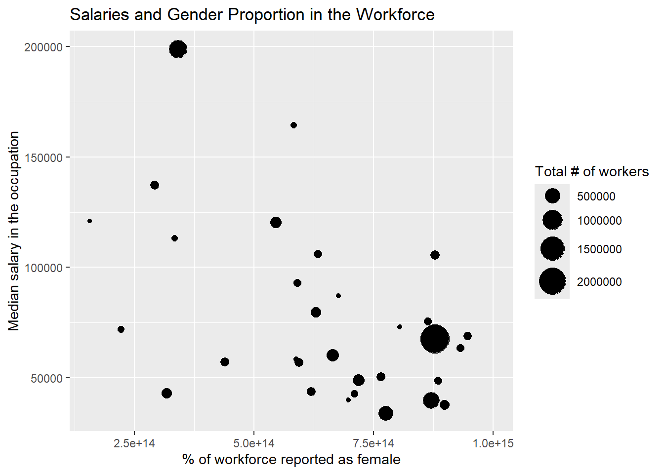
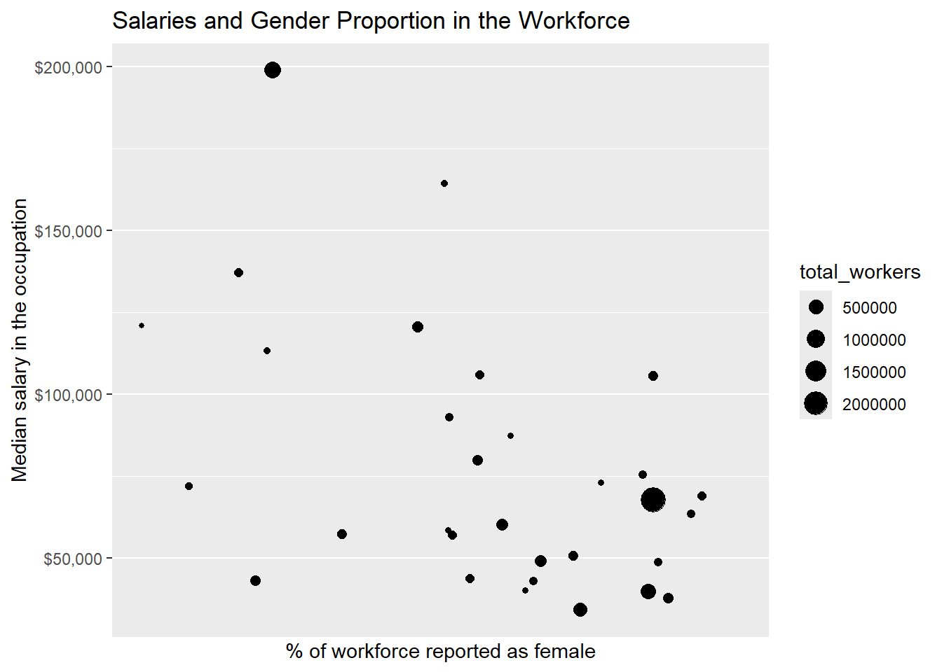
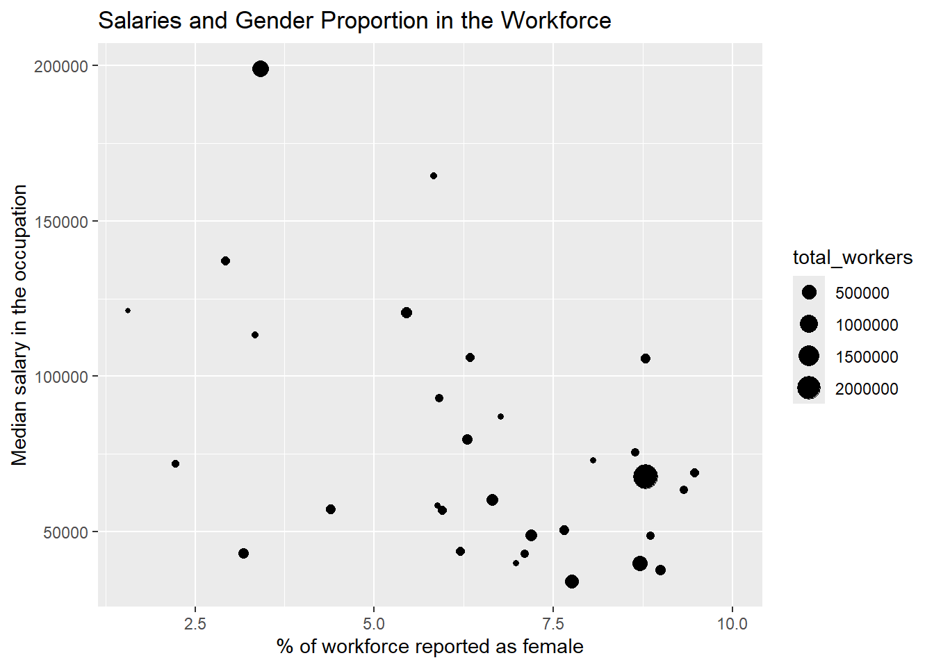
gf_point(median_salary ~ percent_female, size =~ total_workers, data = job_gender,fill ="black", color ="black", alpha =1) %>%gf_labs(title ="Salaries and Gender Proportion in the Workforce",x ="% of workforce reported as female",y ="Median salary in the occupation" ) %>%gf_refine(scale_size_continuous(range =c(1, 10), guide =guide_legend(title ="Total # of workers")))
Warning: Removed 1 row containing missing values or values outside the scale range
(`geom_point()`).
Attempt 2
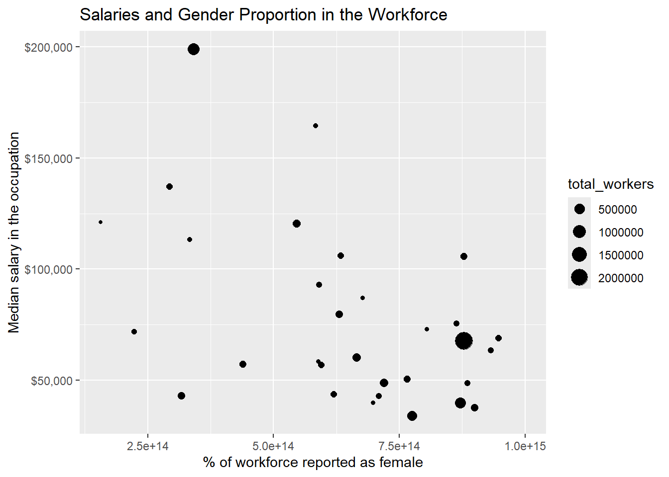
gf_point(median_salary ~ percent_female,size =~ total_workers,data = job_gender,fill ="black",color ="black",alpha =1) %>%gf_labs(title ="Salaries and Gender Proportion in the Workforce",x ="% of workforce reported as female",y ="Median salary in the occupation" ) %>%gf_refine(scale_y_continuous(labels = scales::label_dollar()))
Warning: Removed 1 row containing missing values or values outside the scale range
(`geom_point()`).
In this step, I incorporated the use of the dollar sign for the y-axis scale, ensuring that the monetary values are clearly represented in the graph.
Attempt 3
gf_point(median_salary ~ percent_female, size =~ total_workers, data = job_gender, fill ="black", color ="black", alpha =1) %>%gf_labs(title ="Salaries and Gender Proportion in the Workforce",x ="% of workforce reported as female",y ="Median salary in the occupation" ) %>%gf_refine(scale_x_continuous(labels = scales::percent_format()))
Warning: Removed 1 row containing missing values or values outside the scale range
(`geom_point()`).
I attempted to implement percentages on the x-axis, but all the values ended up displaying as zero.
Attempt 4
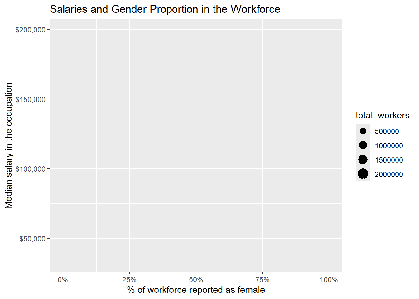
gf_point(median_salary ~ percent_female,size =~ total_workers,data = job_gender,fill ="black",color ="black",alpha =1) %>%gf_labs(title ="Salaries and Gender Proportion in the Workforce",x ="% of workforce reported as female",y ="Median salary in the occupation" ) %>%gf_refine(scale_x_continuous(limits =c(0, 1), labels = scales::percent_format()) )
Warning: Removed 32 rows containing missing values or values outside the scale range
(`geom_point()`).
I tried setting specific limits, but it caused all the bubble plots to shift to 0 percent.
Attempt 5
gf_point(median_salary ~ percent_female,size =~ total_workers,data = job_gender,fill ="black",color ="black",alpha =1) %>%gf_labs(title ="Salaries and Gender Proportion in the Workforce",x ="% of workforce reported as female",y ="Median salary in the occupation") %>%gf_refine(scale_y_continuous(labels = scales::label_dollar()),scale_x_continuous(limits =c(0, 1), labels = scales::percent_format()))
Warning: Removed 32 rows containing missing values or values outside the scale range
(`geom_point()`).
gf_point(median_salary ~ percent_female,size =~ total_workers,data = job_gender,fill ="black",color ="black",alpha =1) %>%gf_labs(title ="Salaries and Gender Proportion in the Workforce",x ="% of workforce reported as female",y ="Median salary in the occupation" ) %>%gf_refine(scale_y_continuous(labels = scales::label_dollar())) %>%gf_refine(scale_x_continuous(limits =c(0, 1), labels = scales::percent_format()) )
Warning: Removed 32 rows containing missing values or values outside the scale range
(`geom_point()`).
Attempt 7
job_gender <- job_gender %>%mutate(percent_female = percent_female /100)gf_point(median_salary ~ percent_female,size =~ total_workers,data = job_gender,fill ="black",color ="black",alpha =1) %>%gf_labs(title ="Salaries and Gender Proportion in the Workforce",x ="% of workforce reported as female",y ="Median salary in the occupation" ) %>%gf_refine(scale_y_continuous(labels = scales::label_dollar())) %>%gf_refine(scale_x_continuous(labels = scales::percent_format()))
Warning: Removed 1 row containing missing values or values outside the scale range
(`geom_point()`).
I attempted to mutate the percent female data, but it still displayed as 0 percent.
Attempt 8
gf_point(median_salary ~ percent_female,size =~ total_workers,data = job_gender,fill ="black",color ="black",alpha =1) %>%gf_labs(title ="Salaries and Gender Proportion in the Workforce",x ="% of workforce reported as female",y ="Median salary in the occupation" ) %>%gf_refine(scale_y_continuous(labels = scales::label_dollar())) %>%gf_refine(scale_x_continuous(breaks =c(0, 0.25, 0.50, 0.75, 1),labels = scales::percent_format() ) )
Warning: Removed 1 row containing missing values or values outside the scale range
(`geom_point()`).
I tried specifying breaks in the data, but the percentages disappeared altogether.
Attempt 9
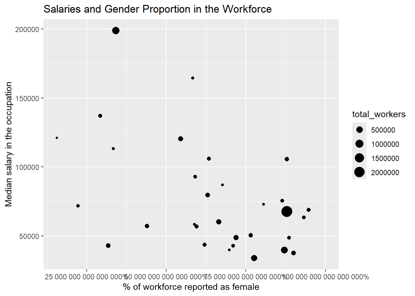
job_gender$percent_female <- job_gender$percent_female *1e2gf_point(median_salary ~ percent_female,size =~ total_workers,data = job_gender,fill ="black",color ="black",alpha =1) %>%gf_labs(title ="Salaries and Gender Proportion in the Workforce",x ="% of workforce reported as female",y ="Median salary in the occupation" ) %>% gf_refine
Warning: Removed 1 row containing missing values or values outside the scale range
(`geom_point()`).
The numbers on the x-axis have changed and no longer match the originals in Attempt 1.
Attempt 10
job_gender$percent_female <- job_gender$percent_female *1e2gf_point(median_salary ~ percent_female,size =~ total_workers,data = job_gender,fill ="black",color ="black",alpha =1) %>%gf_labs(title ="Salaries and Gender Proportion in the Workforce",x ="% of workforce reported as female",y ="Median salary in the occupation" ) %>%gf_refine(scale_y_continuous(labels = scales::label_dollar())) %>%gf_refine(scale_x_continuous(labels = scales::percent_format() ) )
Warning: Removed 1 row containing missing values or values outside the scale range
(`geom_point()`).
I spent about two hours trying to resolve the issue with the data showing 0 percent on the x-axis. Despite multiple attempts—ranging from adjusting the scale, specifying limits, mutating the percentage data, and setting breaks—nothing seemed to work. Each attempt either resulted in all the percentages remaining at 0 or caused the percentages to disappear entirely. Even when I tried different methods, the numbers on the axis shifted, and I still couldn’t get the correct percentages to display. It’s been frustrating, as no matter what I tried, the issue persists, and I haven’t been able to resolve it.
Questions
The graph titled “Salaries and Gender Proportion in the Workforce” seeks to answer the following questions:
1.What is the relationship between salary levels and the proportion of females in various occupations?
( The graph could aim to explore whether occupations with a higher percentage of female workers tend to offer lower salaries compared to male-dominated fields.)
In the dataset, there seems to be a trend where occupations with a higher proportion of female workers tend to offer lower average salaries. For example, jobs such as elementary school teachers (where females represent a large portion of the workforce) have relatively lower wages compared to male-dominated fields like engineering or management, where salaries are significantly higher. This suggests a negative relationship between the proportion of female workers and salary levels.
2.How does gender representation in the workforce affect wage distribution across different job categories?
( It may seek to analyze whether there is a noticeable correlation between the gender composition of an occupation and the wage gap, specifically examining how gender representation impacts salary levels in different sectors.)
The data shows that occupations with more male representation tend to have higher salaries. For example, industries such as construction and technology, which are male-dominated, tend to have higher wages. On the other hand, female-dominated fields like healthcare support or administrative services exhibit lower wage levels, indicating a wage gap between gender representation in different sectors.
3.Which occupations exhibit significant disparities between the proportion of female workers and their salary levels?
( The graph could identify which job categories have high female representation but lower salaries, highlighting potential areas of gender-based wage inequality.)
A significant disparity is observed in roles like nursing, where there is a high proportion of female workers but relatively lower average salaries. Conversely, in occupations such as executive management, which have a low proportion of female workers, the wages are considerably higher. This highlights the wage inequality that exists in certain sectors despite high female representation.
4.Do certain industries show a trend of higher wages for occupations with fewer female workers?
( It may seek to explore whether male-dominated industries offer higher wages compared to female-dominated ones, pointing to the potential for occupational segregation to influence income inequality.)
Yes, industries such as engineering and technology, which are male-dominated, display higher wages. The data indicates that male-dominated fields tend to offer better pay compared to female-dominated occupations, suggesting occupational segregation and its impact on wages.
5.Is there evidence of gender wage gaps in high-paying versus low-paying occupations?
( The graph could aim to determine whether high-paying jobs are more prone to gender wage gaps compared to lower-paying ones, and how these gaps manifest across different sectors.)
Yes, high-paying occupations such as executive management and engineering have a noticeable gender wage gap, with male workers dominating these fields and receiving higher salaries. On the other hand, lower-paying fields like nursing or teaching—which have a higher proportion of female workers—show relatively smaller wage gaps but also lower overall salaries.
Additional Questions
1.What kind of chart is used in the figure?
The chart is a bubble plot (or scatter plot with size variation), where each bubble represents an occupation. The size of the bubbles typically corresponds to the number of workers in that occupation, while the x-axis represents salaries, and the y-axis shows the proportion of female workers in those occupations.
2.What geometries have been used, and to which variables have these geometries been mapped?
The key geometries used in this bubble plot are:
Points (bubbles): Represent occupations.
X-axis: Mapped to salaries (salary levels).
Y-axis: Mapped to the proportion of female workers in each occupation.
Size of bubbles: Mapped to the number of workers in each occupation.
3.Based on this graph, do you think gender plays a role in salaries? What is the trend you see?
Yes, gender seems to play a significant role in salaries. The trend observed is that occupations with higher proportions of female workers tend to have lower salaries. For example, professions dominated by women (e.g., nursing, teaching) exhibit relatively smaller salaries compared to male-dominated fields like engineering or executive management, which have higher wages. This suggests a gender wage gap where male-dominated occupations offer higher pay compared to female-dominated ones.
4.If SALARY, NO_OF_WORKERS, GENDER, OCCUPATION were available in the original dataset, what pre-processing would have been necessary to obtain this plot?
Several preprocessing steps would likely be necessary:
Conversion of Salary Data: Depending on the scale of salary values, some conversion to a common currency/scale might be required for better comparison.
Gender Proportion Calculation: The dataset would need to compute the proportion of female workers (e.g., percentage of female workers relative to the total number of workers in each occupation).
Handling Missing Data: Any missing data in variables such as salary or number of workers would need to be addressed.
Size Mapping: The number of workers would need to be scaled to appropriately map the bubble sizes in the plot, ensuring large and small values are distinguishable.
Aggregating Data: If the data included detailed information about individual workers, it might have been grouped by occupation. This would involve calculating summary statistics such as the average salary, the percentage of female workers, and the total number of workers for each job type.
Inference and Story from the Graph and Data
The graph titled “Salaries and Gender Proportion in the Workforce” provides an insightful view into the relationship between gender proportions in various occupations and the corresponding salary disparities. By analyzing this data, we gain a deeper understanding of how gender representation in the workforce influences salary distribution across different job sectors.
Key Observations
From analyzing the graph and the associated job_gender dataset, I observed the following:
Gender Imbalance in High-Paying Jobs: Occupations with a higher proportion of male workers, such as engineering and technology, tend to have higher median salaries. This indicates that male-dominated industries are often associated with higher compensation, highlighting a disparity in salary distribution across different sectors.
Lower Salaries in Female-Dominated Occupations: On the other hand, jobs with a higher percentage of female workers, such as nursing, teaching, and clerical roles, show significantly lower median salaries. This suggests that occupations traditionally dominated by women often receive lower pay compared to male-dominated fields.
Wage Disparities in Gender-Balanced Roles: Even in occupations where gender representation is relatively balanced, such as healthcare and education, there is still a noticeable gap in median salaries. This reinforces the idea that salary disparity isn’t solely dependent on the proportion of gender but is also influenced by societal and occupational factors.
Insights on Workforce Gender Dynamics
If I were to draw conclusions based on this data, it’s clear that gender continues to play a critical role in shaping salary structures across industries. Investments in gender equity, particularly in improving the salaries of female-dominated sectors, could help bridge the pay gap. Healthcare and education, where salaries remain lower despite more balanced gender representation, should be prioritized in any gender equality effort.
Sector-Specific Insights
Each sector provides different insights into the relationship between gender and salaries:
Male-Dominated Occupations: Roles in engineering, manufacturing, and technology, which are predominantly occupied by men, not only exhibit higher salaries but also reflect the societal value placed on these professions. Addressing this imbalance by encouraging more women to enter these sectors could help reduce the gender pay gap.
Female-Dominated Occupations: Fields such as teaching, nursing, and clerical work are primarily composed of women and tend to have lower salaries. These industries need targeted strategies to increase wages and provide women with equal earning opportunities.
Gender-Balanced Occupations: Even in sectors like healthcare, where gender balance is closer, salary gaps still exist. This suggests that achieving gender parity in representation alone may not be enough to address the underlying pay disparity.
The Power of Data Visualization
This graph effectively visualizes how gender proportions across different occupations impact salary structures, offering key insights for policymakers, businesses, and advocacy groups. The data highlights critical sectors where pay equity efforts should be directed, ensuring equal opportunities and fair compensation regardless of gender. This visualization allows for a more targeted approach to resolving wage disparities and fostering a more inclusive workforce.